import numpy as np
import scipy
import matplotlib.pyplot as plt
from pyLump import Model
import pyExSi

Showcase of the package pyLump

Creating the Model object:

Let’s define a lumped mass (mass-spring-damper) model, shown on the image below, with N degrees of freedom.

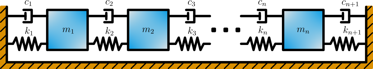
For example, a system with five masses of the same wight connected by springs, where all the springs have the same stiffness value and all the dampers have the same damping coefficient value.

Define the system parameters:

n_dof = 5 # 5 degrees of freedom (5 masses)
mass = 1  # kg
stiffness = 150  # N/m
damping = 2  # N/m/s

We can create an object by calling the Model class. There are 4 different models available with different boundary conditions, which are passed to the object via the boundaries argument. In our case, our model is connected to the rigid surfaces on both sides (boundaries="both"):

model = Model(n_dof=n_dof, mass=mass, stiffness=stiffness, damping=damping, boundaries="both")

Mass, stiffness and damping matrices:

Let’s see the mass, stiffness and damping matrices. To get the matrices we can call the get_mass_matrix(), get_stiffness_matrix() and get_damping_matrix() methods:

print("M = \n", model.get_mass_matrix(), "\n")
print("K = \n", model.get_stiffness_matrix(), "\n")
print("C = \n", model.get_damping_matrix(), "\n")

M =
 [[1. 0. 0. 0. 0.]
 [0. 1. 0. 0. 0.]
 [0. 0. 1. 0. 0.]
 [0. 0. 0. 1. 0.]
 [0. 0. 0. 0. 1.]]

K =
 [[ 300. -150.    0.    0.    0.]
 [-150.  300. -150.    0.    0.]
 [   0. -150.  300. -150.    0.]
 [   0.    0. -150.  300. -150.]
 [   0.    0.    0. -150.  300.]]

C =
 [[ 4. -2.  0.  0.  0.]
 [-2.  4. -2.  0.  0.]
 [ 0. -2.  4. -2.  0.]
 [ 0.  0. -2.  4. -2.]
 [ 0.  0.  0. -2.  4.]]

We can also specify different values for each mass, spring and damper, by passing the arguments as arrays of values. Note that in our case (boundaries="both"), the length of the stiffness and the damping coefficients array, must be N+1 (see the image at the beginning):

mass = np.random.uniform(low=0.2, high=0.5, size=n_dof)  # n_dof masses
stiffness = np.random.uniform(low=400, high=900, size=n_dof+1)  # n_dof+1 springs
damping = np.random.uniform(low=0.1, high=0.3, size=n_dof+1)  # n_dof+1 dampers

Create the object:

model = Model(n_dof=n_dof, mass=mass, stiffness=stiffness, damping=damping, boundaries="both")

Mass, stiffness and damping matrices:

print("M = \n", model.get_mass_matrix(), "\n")
print("K = \n", model.get_stiffness_matrix(), "\n")
print("C = \n", model.get_damping_matrix(), "\n")

M =
 [[0.25766219 0.         0.         0.         0.        ]
 [0.         0.2395301  0.         0.         0.        ]
 [0.         0.         0.29088222 0.         0.        ]
 [0.         0.         0.         0.26284107 0.        ]
 [0.         0.         0.         0.         0.45972559]]

K =
 [[1425.37899259 -651.52023862    0.            0.            0.        ]
 [-651.52023862 1329.41861476 -677.89837614    0.            0.        ]
 [   0.         -677.89837614 1446.62322007 -768.72484393    0.        ]
 [   0.            0.         -768.72484393 1613.33157557 -844.60673164]
 [   0.            0.            0.         -844.60673164 1692.39407393]]

C =
 [[ 0.36391856 -0.1741655   0.          0.          0.        ]
 [-0.1741655   0.3989142  -0.22474869  0.          0.        ]
 [ 0.         -0.22474869  0.51779007 -0.29304138  0.        ]
 [ 0.          0.         -0.29304138  0.56536196 -0.27232057]
 [ 0.          0.          0.         -0.27232057  0.38630849]]

Eigen frequencies:

To get the systems eigen frequencies we can call the get_eig_freq() method:

eig_freq = model.get_eig_freq()
print(eig_freq)

[ 4.32900764  7.94716169 10.9442366  14.19209167 15.88469553]

FRFs and impulse response functions:

Frequency response functions:

To get the frequency response functions of our system we must first define the frequency array (in Hz) with discrete freqeuncy values at which the FRFs are evaluated:

freq = np.linspace(0, 50, 5000)

Now we can calculate the FRFs via get_FRF_matrix() method with freq and frf_method arguments (see tutorial for explanation):

frf_matrix = model.get_FRF_matrix(freq=freq, frf_method="f")

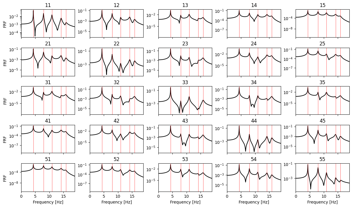
Let’s plot the resulting FRF matrix:

fig, axs = plt.subplots(frf_matrix.shape[0], frf_matrix.shape[1], figsize=(12,7),
                        sharex=True, layout="constrained")

if frf_matrix.shape[0] == 1:
    axs.semilogy(freq, np.abs(frf_matrix[0,0,:]), "k")
    axs.set_title(str(0+1)+str(0+1))
    axs.set_xlabel("Frequency [Hz]")
    axs.set_ylabel("FRF")
    axs.axvline(eig_freq[0], c="r", lw=0.5)
else:
    for i in range(frf_matrix.shape[0]):
        for j in range(frf_matrix.shape[1]):
            axs[i,j].semilogy(freq, np.abs(frf_matrix[i,j,:]), "k")
            axs[i,j].set_title(str(i+1)+str(j+1))
            axs[frf_matrix.shape[1]-1,j].set_xlabel("Frequency [Hz]")
            [axs[i,j].axvline(f_r, c="r", lw=0.5) for f_r in eig_freq]
            axs[i,j].set_xlim(left=0, right=eig_freq[-1]+0.2*eig_freq[-1])
        axs[i,0].set_ylabel("FRF")

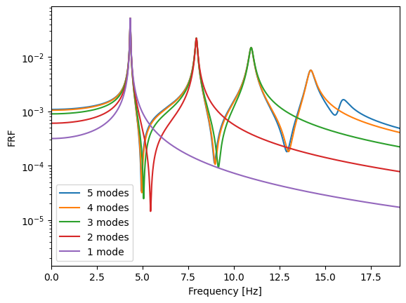
If we choose the state space domain method via modes superposition (frf_method="s"), we can also provide the optional keyword argument n_modes to specify how many modes are considered when caculating FRFs. The comparison is shown below for the first FRF (11 from the FRF matrix above):

frf_nm5 = model.get_FRF_matrix(freq=freq, frf_method="s", n_modes=5)
frf_nm4 = model.get_FRF_matrix(freq=freq, frf_method="s", n_modes=4)
frf_nm3 = model.get_FRF_matrix(freq=freq, frf_method="s", n_modes=3)
frf_nm2 = model.get_FRF_matrix(freq=freq, frf_method="s", n_modes=2)
frf_nm1 = model.get_FRF_matrix(freq=freq, frf_method="s", n_modes=1)


plt.semilogy(freq, np.abs(frf_nm5[0,0,:]), label="5 modes")
plt.semilogy(freq, np.abs(frf_nm4[0,0,:]), label="4 modes")
plt.semilogy(freq, np.abs(frf_nm3[0,0,:]), label="3 modes")
plt.semilogy(freq, np.abs(frf_nm2[0,0,:]), label="2 modes")
plt.semilogy(freq, np.abs(frf_nm1[0,0,:]), label="1 mode")
plt.xlim(left=0, right=eig_freq[-1]+0.2*eig_freq[-1])
plt.legend()
plt.xlabel("Frequency [Hz]")
plt.ylabel("FRF");

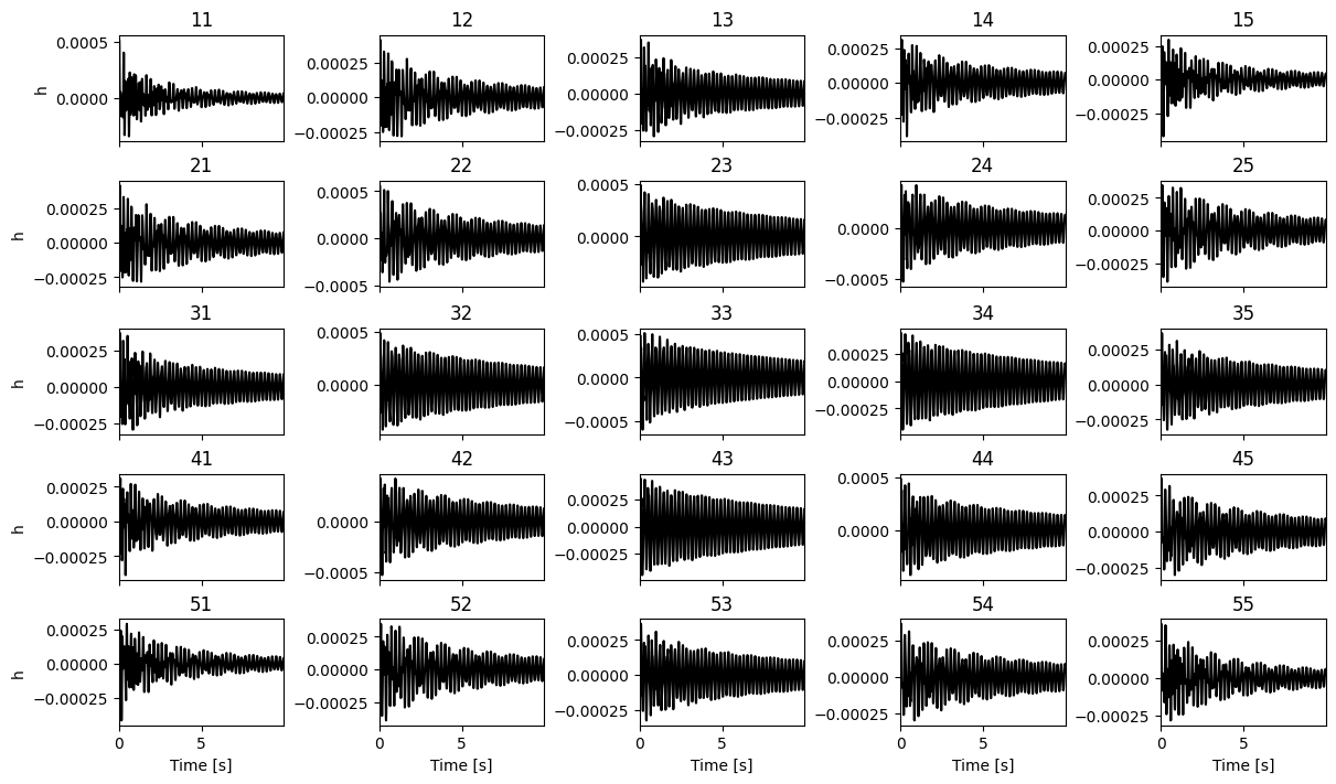
Impulse response functions:

We can calculate the impulse response functions via get_IRF_matrix() method. We can also obtain the time axis with return_t_axis argument:

irf_matrix, time = model.get_IRF_matrix(freq=freq, frf_method="f", return_t_axis=True)

Let’s plot the resulting impulse reponse functions matrix:

fig, axs = plt.subplots(irf_matrix.shape[0], irf_matrix.shape[1], figsize=(12,7),
                        sharex=True, layout="constrained")

if irf_matrix.shape[0] == 1:
    axs.plot(time, irf_matrix[0,0,:], "k")
    axs.set_title(str(0+1)+str(0+1))
    axs.set_xlabel("Time [s]")
    axs.set_ylabel("h")
else:
    for i in range(irf_matrix.shape[0]):
        for j in range(irf_matrix.shape[1]):
            axs[i,j].plot(time, irf_matrix[i,j,:], "k")
            axs[i,j].set_xlim(left=0, right=time[-1]/10)
            axs[i,j].set_title(str(i+1)+str(j+1))
            axs[irf_matrix.shape[1]-1,j].set_xlabel("Time [s]")
        axs[i,0].set_ylabel("h")

Calculating response

We can calculate the response of the masses via frequency response functions (multiplication in frequency domain - domain="f") or via impulse response functions (convolution in time domain - domain="t") with get_response() method. In this example we wil show how to obtain response via FRFs (domain="f").

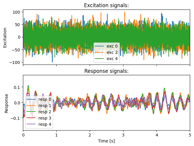
Let’s define our excitation signals with pyExSi package, their sampling rate and duration and specify which masses (excitation degrees of freedom) are the signals applied to. We must also define which responses we want to calculate. If that is not provided, the responses of all masses are calculated:

exc_dof = [0, 2, 4]  # first third and the last mass are excited
sampling_rate = 1000
T = 20  # duration of the excitation signals
resp_dof = [0, 1, 2, 3, 4]  # calculate the responses of all masses

exc = np.zeros((len(exc_dof), int(T*sampling_rate)), dtype=float)

for i in range(len(exc_dof)):
    exc[i] = 100 * pyExSi.normal_random(N=int(T*sampling_rate))

Calculate response:

resp, time = model.get_response(exc_dof=exc_dof, exc=exc, sampling_rate=sampling_rate,
                                resp_dof=resp_dof, domain="f", frf_method="f",
                                return_matrix=False, return_t_axis=True, return_f_axis=False)

Let’s plot the excitation and the obtained response signals:

fig, axs = plt.subplots(2, 1, sharex=True, layout="constrained")

for i in range(exc.shape[0]):
    axs[0].plot(time, exc[i], label="exc "+str(exc_dof[i]))

for i in range(resp.shape[0]):
    axs[1].plot(time, resp[i], label="resp "+str(resp_dof[i]))

axs[0].set_title("Excitation signals:")
axs[1].set_title("Response signals:")
axs[1].set_ylabel('Response')
axs[0].set_ylabel('Excitation')
axs[1].set_xlabel('Time [s]');
axs[0].set_xlim(0,5)
axs[0].legend()
axs[1].legend();

Other methods

There are also other methods available, for example, we can obtain eigen values and their conjugate pairs via get_eig_val() method. The same goes for eigen vectors via get_eig_vec() method.

We can aslo obtain viscous damping ratios of our system via get_damping_ratios() method:

damping_ratios = model.get_damping_ratios()
print(damping_ratios)

[0.00301382 0.00650376 0.00987437 0.01329006 0.01656951]